Single Layer Feed Forward Network Having Multiple Output Neurons Python Code

Machine Learning, Scholarly, Tutorial
Building Neural Networks with Python Code and Math in Detail — II
The second part of our tutorial on neural networks from scratch. From the math behind them to step-by-step implementation case studies in Python. Launch the samples on Google Colab.
Last updated January 7, 2021
Author(s): Pratik Shukla, Roberto Iriondo
In the first part of our tutorial on neural networks, we explained the basic concepts about neural networks, from the math behind them to implementing neural networks in Python without any hidden layers. We showed how to make satisfactory predictions even in case scenarios where we did not use any hidden layers. However, there are several limitations to single-layer neural networks.
In this tutorial, we will dive in-depth into the limitations and advantages of using neural networks in machine learning. We will show how to implement neural nets with hidden layers and how these lead to a higher accuracy rate on our predictions, along with implementation samples in Python on Google Colab.
Index:
- Limitations and advantages of neural networks
- How to select several neurons in a hidden layer.
- The general structure of an artificial neural network (ANN).
- Implementation of a multilayer neural network in Python.
- Comparison with a single-layer neural network.
- Non-linearly separable data with a neural network.
- Conclusion.
📚 Check out our editorial recommendations on the best machine learning books. 📚
1. Limitations and Advantages of Neural Networks
Limitations of single-layer neural networks:
- They can only represent a limited set of functions. If we have been training a model that uses complicated functions (which is the general case), then using a single layer neural network can lead to low accuracy in our prediction rate.
- They can only predict linearly separable data. If we have non-linear data, then training our single-layer neural network will lead to low accuracy in our prediction rate.
- Decision boundaries for single-layer neural networks must be in the hyperplane, which means that if our data distributes in 3 dimensions, then our decision boundary must be in 2 dimensions.
To overcome such limitations, we use hidden layers in our neural networks.
Advantages of single-layer neural networks:
- Single-layer neural networks are easy to set up.
- Single-layer neural networks take less time to train compared to a multi-layer neural network.
- Single-layer neural networks have explicit links to statistical models.
- The outputs in single layer neural networks are weighted sums of inputs. It means that we can interpret the output of a single layer neural network feasibly.
Advantages of multilayer neural networks:
- They construct more extensive networks by considering layers of processing units.
- They can be used to classify non-linearly separable data.
- Multilayer neural networks are more reliable compared to single-layer neural networks.
2. How to select several neurons in a hidden layer?
There are many methods for determining the correct number of neurons to use in the hidden layer. We will see a few of them here.
- The number of hidden nodes should be less than twice the size of the nodes in the input layer.
For example: If we have 2 input nodes, then our hidden nodes should be less than 4.
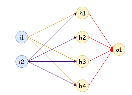
a. 2 inputs, 4 hidden nodes:
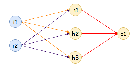
b. 2 inputs, 3 hidden nodes:
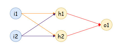
c. 2 inputs, 2 hidden nodes:
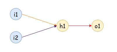
d. 2 inputs, 1 hidden node:
- The number of hidden nodes should be 2/3 the size of input nodes, plus the size of the output node.
For example: If we have 2 input nodes and 1 output node then the hidden nodes should be = floor(2*2/3 + 1) = 2
a. 2 inputs, 2 hidden nodes:

- The number of hidden nodes should be between the size of input nodes and output nodes.
For example: If we have 3 input nodes and 2 output nodes, then the hidden nodes should be between 2 and 3.
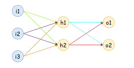
a. 3 inputs, 2 hidden nodes, 2 outputs:
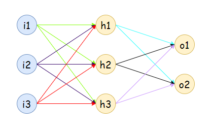
b. 3 inputs, 3 hidden nodes, 2 outputs:
How many weight values do we need?
- For a hidden layer: Number of inputs * No. of hidden layer nodes
- For an output layer: Number of hidden layer nodes * No. of outputs
3. The General Structure of an Artificial Neural Network (ANN):
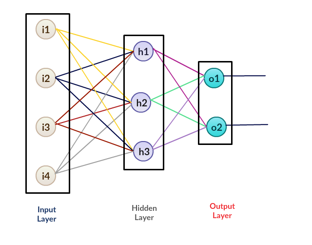
Summarization of an artificial neural network:
- Take inputs.
- Add bias (if required).
- Assign random weights in the hidden layer and the output layer.
- Run the code for training.
- Find the error in prediction.
- Update the weight values of the hidden layer and output layer by gradient descent algorithm.
- Repeat the training phase with updated weights.
- Make predictions.
Execution of multilayer neural networks:
After reading the first article, we saw that we had only 1 phase of execution there. In that phase, we find the updated weight values and rerun the code to achieve minimum error. However, things are a little spicy here. The execution in a multilayer neural network takes place in two-phase. In phase-1, we update the values of weight_output (weight values for output layer), and in phase-2, we update the value of weight_hidden ( weight values for the hidden layer ). Phase-1 is similar to that of a neural network without any hidden layers.
Execution in phase-1:
To find the derivative, we are going to use in gradient descent algorithm to update the weight values. Here we are not going to derive the derivatives for those functions we already did in part -1 of neural network.
In this phase, our goal is to find the weight values for the output layer. Here we are going to calculate the change in error concerning the change in output weight.
We first define some terms we are going to use in these derivatives:
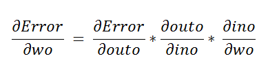
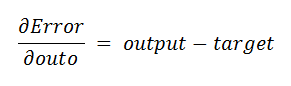
a. Finding the first derivative:
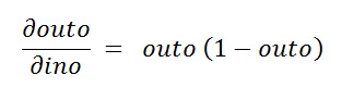
b. Finding the second derivative:
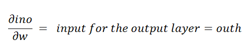
c. Finding the third derivative:
Notice that we already derived these derivatives in the first part of our tutorial.
Execution in phase-2:
In phase-1, we find the updated weight for the output layer. In the second phase, we need to find the updated weights for the hidden layer. Hence, find how the change in hidden weight affects the change in error value.
Represented as:
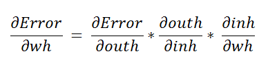
a. Finding the first derivative:
Here we are going to use the chain rule to find the derivative.
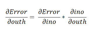
Using the chain rule again.
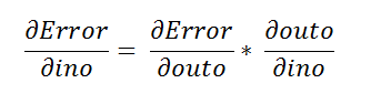
The step below is similar to what we did in the first part of our tutorial on neural networks.
b. Finding the second derivative:
c. Finding the third derivative:
4. Implementation of a multilayer neural network in Python
📚 Multilayer neural network: A neural network with a hidden layer 📚 For more definitions, check out our article in terminology in machine learning.
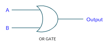
Below we are going to implement the "OR" gate without the bias value. In conclusion, adding hidden layers in a neural network helps us achieve higher accuracy in our models.
Representation:
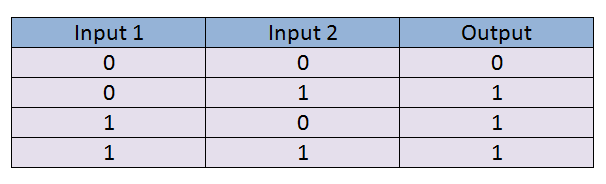
Truth-Table:
Neural Network:
Notice that here we have 2 input features and 1 output feature. In this neural network, we are going to use 1 hidden layer with 3 nodes.
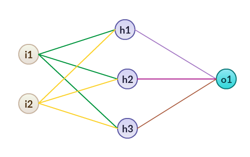
Graphical representation:
Implementation in Python:
Below, we are going to implement our neural net with hidden layers step by step in Python, let's code:
a. Import required libraries:
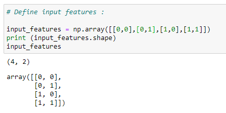
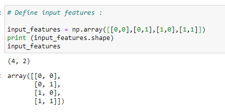
b. Define input features:
Next, we take input values for which we want to train our neural network. We can see that we have taken two input features. On tangible data sets, the value of input features is mostly high.
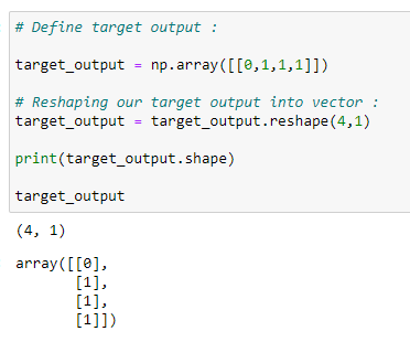
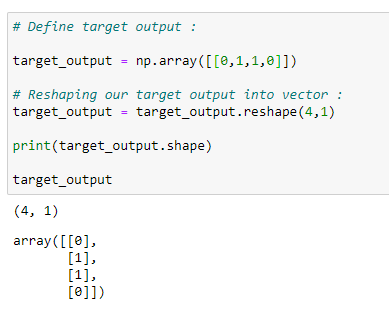
c. Define target output values:
For the input features, we want to have a specific output for specific input features. It is called the target output. We are going to train the model that gives us the target output for our input features.
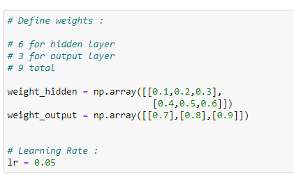
d. Assign random weights:
Next, we are going to assign random weights to the input features. Note that our model is going to modify these weight values to be optimal. At this point, we are taking these values randomly. Here we have two layers, so we have to assign weights for them separately.
The other variable is the learning rate. We are going to use the learning rate (LR) in a gradient descent algorithm to update the weight values. Generally, we keep LR as low as possible so that we can achieve a minimal error rate.
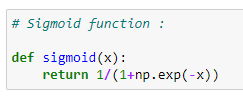
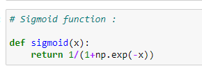
e. Sigmoid function:
Once we have our weight values and input features, we are going to send it to the main function that predicts the output. Notice that our input features and weight values can be anything, but here we want to classify data, so we need the output between 0 and 1. For such output, we are going to use a sigmoid function.
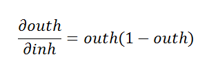
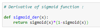
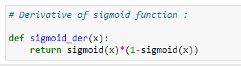
f. Sigmoid function derivative:
In a gradient descent algorithm, we need the derivative of the sigmoid function.
g. The main logic for predicting output and updating the weight values:
We are going to understand the following code step-by-step.
How does it work?
a. First of all, we run the above code 2,00,000 times. Keep in mind that if we only run this code a few times, then it is probable that we will have a higher error rate. Therefore, we update the weight values 10,000 times to reach the optimal value possible.
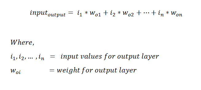
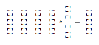
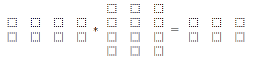
b. Next, we find the input for the hidden layer. Defined by the following formula:
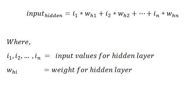
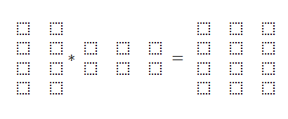
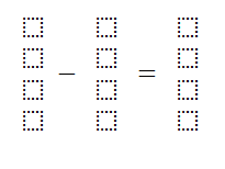
We can also represent it as matrices to understand in a better way.
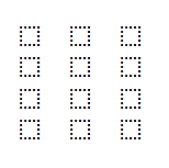
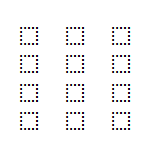
The first matrix here is input features with size (4*2), and the second matrix is weight values for a hidden layer with size (2*3). So the resultant matrix will be of size (4*3).
The intuition behind the final matrix size:
The row size of the final matrix is the same as the row size of the first matrix, and the column size of the final matrix is the same as the column size of the second matrix in multiplication (dot product).
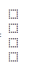
In the representation below, each of those boxes represents a value.
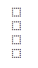
c. Afterward, we have an input for the hidden layer, and it is going to calculate the output by applying a sigmoid function. Below is the output of the hidden layer:
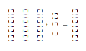
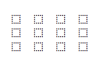
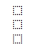
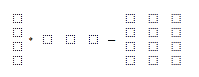
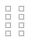
d. Next, we multiply the output of the hidden layer with the weight of the output layer:
The first matrix shows the output of the hidden layer, which has a size of (4*3). The second matrix represents the weight values of the output layer,
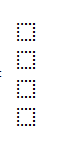
e. Afterward, we calculate the output of the output layer by applying a sigmoid function. It can also be represented in matrix form as follows.
f. Now that we have our predicted output, we find the mean squared between target output and predicted output.
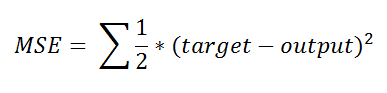
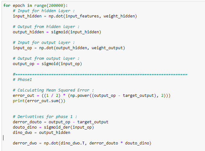
g. Next, we begin the first phase of training. In this step, we update the weight values for the output layer. We need to find out how much the output weights affect the error value. To update the weights, we use a gradient descent algorithm. Notice that we have already found the derivatives we will use during the training phase.

g.a. Matrix representation of the first derivative. Matrix size (4*1).
derror_douto = output_op -target_output
g.b. Matrix representation of the second derivative. Matrix size (4*1).
dout_dino = sigmoid_der(input_op)
g.c. Matrix representation of the third derivative. Matrix size (4*3).
dino_dwo = output_hidden

g.d. Matrix representation of transpose of dino_dwo. Matrix size (3*4).
g.e. Now, we are going to find the final matrix of output weight. For a detailed explanation of this step, please check out our previous tutorial. The matrix size will be (3*1), which is the same as the output_weight matrix.
Hence, we have successfully find the derivative values. Next, we update the weight values accordingly with the help of a gradient descent algorithm.
Nonetheless, we also have to find the derivative for phase-2. Let's first find that, and then we will update the weights for both layers in the end.
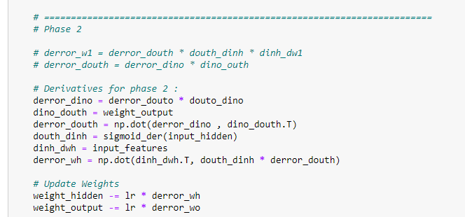
h. Phase -2. Updating the weights in the hidden layer.
Since we have already discussed how we derived the derivative values, we are just going to see matrix representation for each of them to understand it better. Our goal here is to find the weight matrix for the hidden layer, which is of size (2*3).
h.a. Matrix representation for the first derivative.
derror_dino = derror_douto * douto_dino
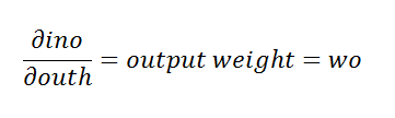
h.b. Matrix representation for the second derivative.
dino_douth = weight_output
h.c. Matrix representation for the third derivative.
derror_douth = np.dot(derror_dino , dino_douth.T)
h.d. Matrix representation for the fourth derivative.
douth_dinh = sigmoid_der(input_hidden)
h.e. Matrix representation for the fifth derivative.
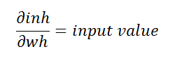
dinh_dwh = input_features
h.f. Matrix representation for the sixth derivative.
derror_dwh = np.dot(dinh_dwh.T, douth_dinh * derror_douth)
Notice that our goal was to find a hidden weight matrix with the size of (2*3). Furthermore, we have successfully managed to find it.
h.g. Updating the weight values :
We will use the gradient descent algorithm to update the values. It takes three parameters.
- The original weight: we already have it.
- The learning rate (LR): we assigned it the value of 0.05.
- The derivative: Found on the previous step.
Gradient descent algorithm:
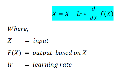
Since we have all of our parameter values, this will be a straightforward operation. First, we are updating the weight values for the output layer, and then we are updating the weight values for the hidden layer.
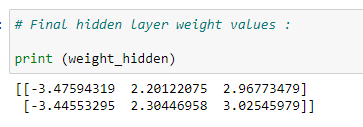
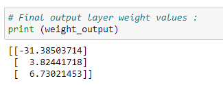
i. Final weight values:
Below, we show the updated weight values for both layers — our prediction bases on these values.
j. Making predictions:
j.a. Prediction for (1,1).
Target output = 1
Explanation:
First of all, we are going to take the input values for which we want to predict the output. The "result1" variable stores the value of the dot product of input variables and hidden layer weight. We obtain the output by applying a sigmoid function, the result stores in the result2 variable. Such is the input feature for the output layer. We calculate the input for the output layer by multiplying input features with output layer weight. To find the final output value, we take the sigmoid value of that.
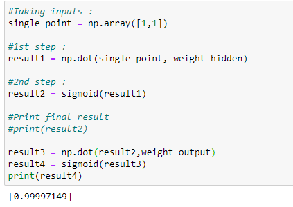
Notice that the predicted output is very close to 1. So we have managed to make accurate predictions.
j.b. Prediction for (0,0).
Target output = 0
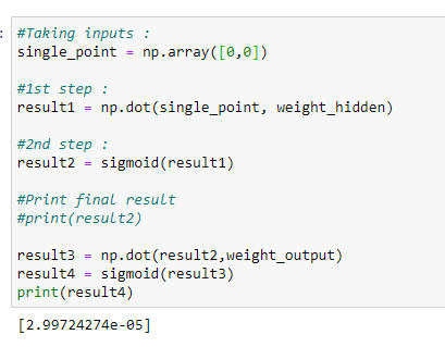
Note that the predicted output is very close to 0, which indicates the success rate of our model.
k. Final error value :
After 200,000 iterations, we have our final error value — the lower the error, the higher the accuracy of the model.

As shown above, we can see that the error value is 0.0000000189. This value is the final error value in prediction after 200,000 iterations.
Putting it all together:
# Import required libraries :
import numpy as np# Define input features :
input_features = np.array([[0,0],[0,1],[1,0],[1,1]])
print (input_features.shape)
print (input_features)# Define target output :
target_output = np.array([[0,1,1,1]])# Reshaping our target output into vector :
target_output = target_output.reshape(4,1)
print(target_output.shape)
print (target_output)# Define weights :
# 6 for hidden layer
# 3 for output layer
# 9 totalweight_hidden = np.array([[0.1,0.2,0.3],
[0.4,0.5,0.6]])
weight_output = np.array([[0.7],[0.8],[0.9]])# Learning Rate :
lr = 0.05# Sigmoid function :
def sigmoid(x):
return 1/(1+np.exp(-x))# Derivative of sigmoid function :
def sigmoid_der(x):
return sigmoid(x)*(1-sigmoid(x))for epoch in range(200000):
# Input for hidden layer :
input_hidden = np.dot(input_features, weight_hidden) # Output from hidden layer :
output_hidden = sigmoid(input_hidden)
# Input for output layer :
input_op = np.dot(output_hidden, weight_output)
# Output from output layer :
output_op = sigmoid(input_op)#==========================================================
# Phase1
# Calculating Mean Squared Error :
error_out = ((1 / 2) * (np.power((output_op — target_output), 2)))
print(error_out.sum())
# Derivatives for phase 1 :
derror_douto = output_op — target_output
douto_dino = sigmoid_der(input_op)
dino_dwo = output_hiddenderror_dwo = np.dot(dino_dwo.T, derror_douto * douto_dino)#===========================================================
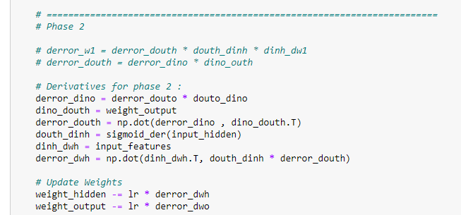
# Phase 2
# derror_w1 = derror_douth * douth_dinh * dinh_dw1
# derror_douth = derror_dino * dino_outh
# Derivatives for phase 2 :
derror_dino = derror_douto * douto_dino
dino_douth = weight_output
derror_douth = np.dot(derror_dino , dino_douth.T)
douth_dinh = sigmoid_der(input_hidden)
dinh_dwh = input_features
derror_wh = np.dot(dinh_dwh.T, douth_dinh * derror_douth)# Update Weights
weight_hidden -= lr * derror_wh
weight_output -= lr * derror_dwo
# Final hidden layer weight values :
print (weight_hidden)# Final output layer weight values :
print (weight_output)# Predictions :#Taking inputs :
single_point = np.array([1,1])
#1st step :
result1 = np.dot(single_point, weight_hidden)
#2nd step :
result2 = sigmoid(result1)
#3rd step :
result3 = np.dot(result2,weight_output)
#4th step :
result4 = sigmoid(result3)
print(result4)#=================================================
#Taking inputs :
single_point = np.array([0,0])
#1st step :
result1 = np.dot(single_point, weight_hidden)
#2nd step :
result2 = sigmoid(result1)
#3rd step :
result3 = np.dot(result2,weight_output)
#4th step :
result4 = sigmoid(result3)
print(result4)#=====================================================
#Taking inputs :
single_point = np.array([1,0])
#1st step :
result1 = np.dot(single_point, weight_hidden)
#2nd step :
result2 = sigmoid(result1)
#3rd step :
result3 = np.dot(result2,weight_output)
#4th step :
result4 = sigmoid(result3)
print(result4)
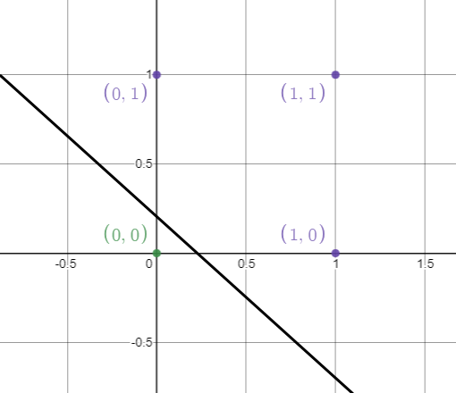
Below, notice that the data we used in this example was linearly separable, which means that by a single line, we can classify outputs with 1 value and outputs with 0 values.
Launch it on Google Colab:
5. Comparison with a single-layer neural network
Notice that we did not use bias value here. Now let's have a quick look at the neural network without hidden layers for the same input features and target values. What we are going to do is find the final error rate and compare it. Since we have already implemented the code in our previous tutorial, for this purpose, we are going to analyze it quickly. [2]
The final error value for the following code is:
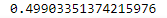
As we can see, the error value is way too high compared to the error we found in our neural network implementation with hidden layers, making it one of the main reasons to use hidden layers in a neural network.
                # Import required libraries :
import numpy as np# Define input features :
input_features = np.array([[0,0],[0,1],[1,0],[1,1]])
print (input_features.shape)
print (input_features)# Define target output :
target_output = np.array([[0,1,1,1]])# Reshaping our target output into vector :
target_output = target_output.reshape(4,1)
print(target_output.shape)
print (target_output)# Define weights :
weights = np.array([[0.1],[0.2]])
print(weights.shape)
print (weights)# Define learning rate :
lr = 0.05# Sigmoid function :
def sigmoid(x):
                  return 1/(1+np.exp(-x))# Derivative of sigmoid function :
def sigmoid_der(x):
                  return sigmoid(x)*(1-sigmoid(x))# Main logic for neural network :
# Running our code 10000 times :for epoch in range(10000):
                  inputs = input_features#Feedforward input :
                  pred_in = np.dot(inputs, weights)#Feedforward output :
                  pred_out = sigmoid(pred_in)#Backpropogation
                  #Calculating error
                  error = pred_out - target_output
                  x = error.sum()                        #Going with the formula :
                    print(x)                                          #Calculating derivative :
                    dcost_dpred = error
                    dpred_dz = sigmoid_der(pred_out)                                          #Multiplying individual derivatives :
                    z_delta = dcost_dpred * dpred_dz#Multiplying with the 3rd individual derivative :
                    inputs = input_features.T
                    weights -= lr * np.dot(inputs, z_delta)#Predictions :#Taking inputs :
single_point = np.array([1,0])
#1st step :
result1 = np.dot(single_point, weights)
#2nd step :
result2 = sigmoid(result1)
#Print final result
print(result2)#====================================
#Taking inputs :
single_point = np.array([0,0])
#1st step :
result1 = np.dot(single_point, weights)
#2nd step :
result2 = sigmoid(result1)
#Print final result
print(result2)#===================================
#Taking inputs :
single_point = np.array([1,1])
#1st step :
result1 = np.dot(single_point, weights)
#2nd step :
result2 = sigmoid(result1)
#Print final result
print(result2)
Launch it on Google Colab:
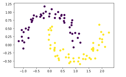
6. Non-linearly separable data with a neural network
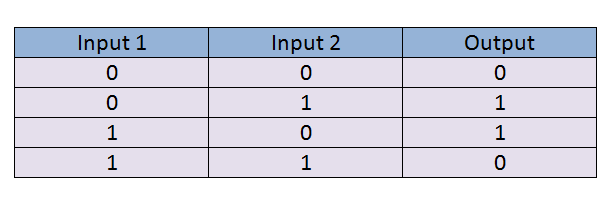
In this example, we are going to take a dataset that cannot be separated by a single straight line. If we try to separate it by a single line, then one or many outputs may be misclassified, and we will have a very high error. Therefore we use a hidden layer to resolve this issue.
Input Table:
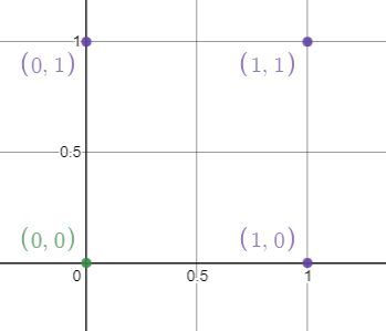
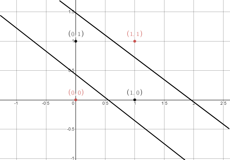
Graphical Representation Of Data Points :
As shown below, we represent the data on the coordinate plane. Here notice that we have 2 colored dots (black and red). If we try to draw a single line, then the output is going to be misclassified.
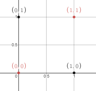
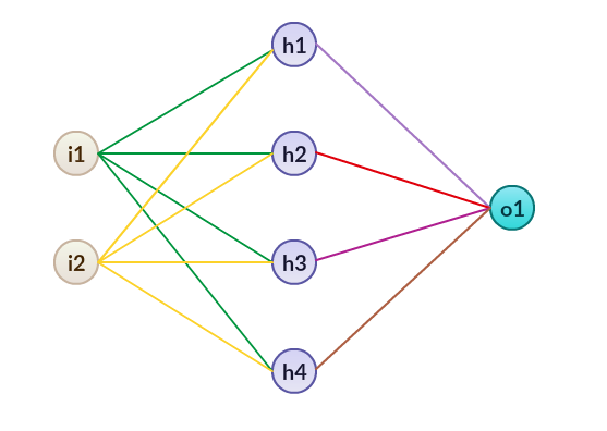
As figure 59 shows, we have 2 inputs and 1 output. In this example, we are going to use 4 hidden perceptrons. The red dots have an output value of 0, and the black dots have an output value of 1. Therefore, we cannot simply classify them using a single straight line.
Neural Network:
Implementation in Python:
a. Import required libraries:
b. Define input features:
c. Define the target output:
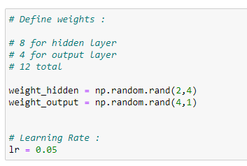
d. Assign random weight values:
On figure 64, notice that we are using NumPy's library random function to generate random values.
numpy.random.rand(x,y): Here x is the number of rows, and y is the number of columns. It generates output values over [0,1). It means 0 is included, but 1 is not included in the value generation.
e. Sigmoid function:
f. Finding the derivative with a sigmoid function:
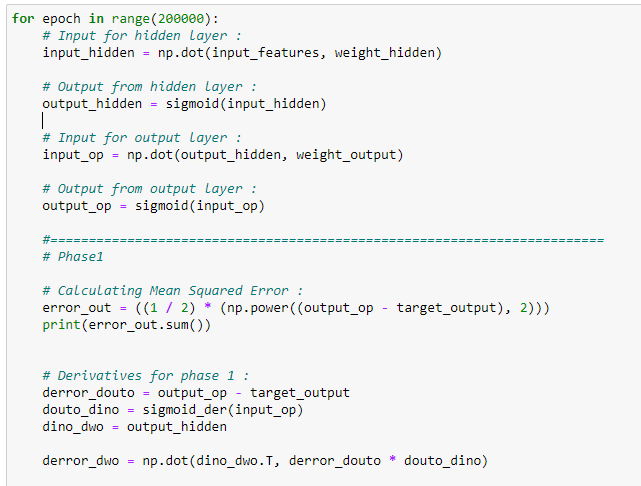
g. Training our neural network:
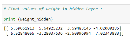
h. Weight values of hidden layer:
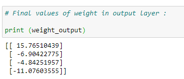
i. Weight values of output layer:
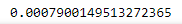
j. Final error value :
After training our model for 200,000 iterations, we finally achieved a low error value.
k. Making predictions from the trained model :
k.a. Predicting output for (0.5, 2).
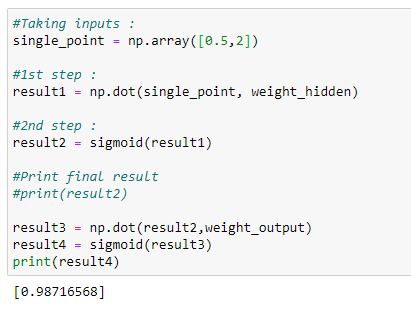
The predicted output is closer to 1.
k.b. Predicting output for (0, -1)
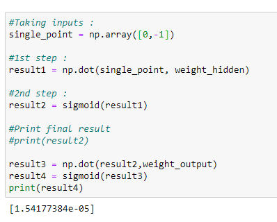
The predicted output is very near to 0.
k.c. Predicting output for (0, 5)
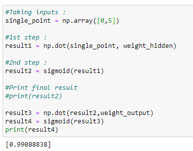
The predicted output is close to 1.
k.d. Predicting output for (1, 1.2)
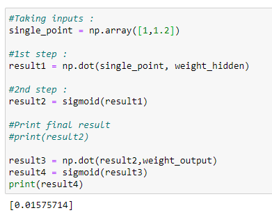
The predicted output is close to 0.
Based on the output values, our model has done a high-grade job of predicting values.
We can separate our data in the following way as shown in Figure 76. Note that this is not the only possible way to separate these values.
Therefore to conclude, using a hidden layer on our neural networks helps us reducing the error rate when we have non-linearly separable data. Even though the training time extends, we have to remember that our goal is to make high accuracy predictions, and such will be satisfied.
Putting it all together:
                # Import required libraries :
import numpy as np# Define input features :
input_features = np.array([[0,0],[0,1],[1,0],[1,1]])
print (input_features.shape)
print (input_features)# Define target output :
target_output = np.array([[0,1,1,0]])# Reshaping our target output into vector :
target_output = target_output.reshape(4,1)
print(target_output.shape)
print (target_output)# Define weights :
# 8 for hidden layer
# 4 for output layer
# 12 total
weight_hidden = np.random.rand(2,4)
weight_output = np.random.rand(4,1)# Learning Rate :
lr = 0.05# Sigmoid function :
def sigmoid(x):
                  return 1/(1+np.exp(-x))# Derivative of sigmoid function :
def sigmoid_der(x):
                  return sigmoid(x)*(1-sigmoid(x))# Main logic :
for epoch in range(200000):
                  # Input for hidden layer :
                  input_hidden = np.dot(input_features, weight_hidden)                     # Output from hidden layer :
                    output_hidden = sigmoid(input_hidden)                                       # Input for output layer :
                    input_op = np.dot(output_hidden, weight_output)                                       # Output from output layer :
                    output_op = sigmoid(input_op)#========================================================================
                    # Phase1                                       # Calculating Mean Squared Error :
                    error_out = ((1 / 2) * (np.power((output_op — target_output), 2)))
                    print(error_out.sum())                                        # Derivatives for phase 1 :
                    derror_douto = output_op — target_output
                    douto_dino = sigmoid_der(input_op)
                    dino_dwo = output_hiddenderror_dwo = np.dot(dino_dwo.T, derror_douto * douto_dino)# ========================================================================
                    # Phase 2# derror_w1 = derror_douth * douth_dinh * dinh_dw1
                    # derror_douth = derror_dino * dino_outh                                       # Derivatives for phase 2 :
                    derror_dino = derror_douto * douto_dino
                    dino_douth = weight_output
                    derror_douth = np.dot(derror_dino , dino_douth.T)
                    douth_dinh = sigmoid_der(input_hidden)
                    dinh_dwh = input_features
                    derror_dwh = np.dot(dinh_dwh.T, douth_dinh * derror_douth)# Update Weights
                    weight_hidden -= lr * derror_dwh
                    weight_output -= lr * derror_dwo                                       # Final values of weight in hidden layer :
print (weight_hidden)# Final values of weight in output layer :
print (weight_output)#Taking inputs :
single_point = np.array([0,-1])
#1st step :
result1 = np.dot(single_point, weight_hidden)
#2nd step :
result2 = sigmoid(result1)
#3rd step :
result3 = np.dot(result2,weight_output)
#4th step :
result4 = sigmoid(result3)
print(result4)#Taking inputs :
single_point = np.array([0,5])
#1st step :
result1 = np.dot(single_point, weight_hidden)
#2nd step :
result2 = sigmoid(result1)
#3rd step :
result3 = np.dot(result2,weight_output)
#4th step :
result4 = sigmoid(result3)
print(result4)#Taking inputs :
single_point = np.array([1,1.2])
#1st step :
result1 = np.dot(single_point, weight_hidden)
#2nd step :
result2 = sigmoid(result1)
#3rd step :
result3 = np.dot(result2,weight_output)
#4th step :
result4 = sigmoid(result3)
print(result4)
Launch it on Google Colab:
7. Conclusion
- Neural networks can learn from their mistakes, and they can produce output that is not limited to the inputs provided to them.
- Inputs store in its networks instead of a database.
- These networks can learn from examples, and we can predict the output for similar events.
- In case of failure of one neuron, the network can detect the fault and still produce output.
- Neural networks can perform multiple tasks in parallel processes.

DISCLAIMER: The views expressed in this article are those of the author(s) and do not represent the views of Carnegie Mellon University, nor other companies (directly or indirectly) associated with the author(s). These writings do not intend to be final products, yet rather a reflection of current thinking, along with being a catalyst for discussion and improvement.
Published via Towards AI
Citation
For attribution in academic contexts, please cite this work as:
Shukla, et al., "Building Neural Networks with Python Code and Math in Detail — II", Towards AI, 2020 BibTex citation:
                @article{pratik_iriondo_2020,
                  title={Building Neural Networks with Python Code and Math in Detail — II},
                  url={https://towardsai.net/building-neural-nets-with-python},
                  journal={Towards AI},
                  publisher={Towards AI Co.},
                  author={Pratik, Shukla and Iriondo, Roberto},
                  year={2020},
                  month={Jun}
}
📚 Are you new to machine learning? Check out an overview of machine learning algorithms for beginners with code examples in Python 📚
References:
[1] Stats Stack Exchange, https://stats.stackexchange.com
[2] Neural Networks from Scratch with Python Code and Math in Detail — I, Pratik Shukla, Roberto Iriondo, https://towardsai.net/neural-networks-with-python
Source: https://pub.towardsai.net/building-neural-networks-with-python-code-and-math-in-detail-ii-bbe8accbf3d1